Algebra I: Lesson Plan * 11/20/2006

Quickstart
p.375
#50 - 54

Chapter 7: Systems of Equations and Inequalities
7-1: Solving Systems by Graphing
Objectives:
(MA.C.3.4.2) To graph, apply, and verify properties of two- and three-dimensional figures
(MA.C.3.4.2, MA.D.2.4.2) To analyze systems using slope, to use systems of equations to solve real-world problems.

Example 1 - Solving a system of equations

Example 3 - Systems with no solution

Example 4 - system with infinitely many solutions

Watch the video tutorial

Homework
p.343-344
# 3 - 24 x 3's, 43 - 45 ALL

Algebra I: Lesson Plan * 11/17/2006

Quickstart
Mini - BAT Assessment
Strand E, Standard 3, Form A
Experiments
MA.E.3.4.1, MA.E.3.4.2

Reteaching
Strand E, Standard 1
Data Analysis
A useful website about reading Venn Diagrams.


Strand E, Standard 2
Combinations and Permutations
Watch a video tutorial about finding the probability of independent events.

Lesson
7-1 Solving Systems by Graphing
Objective
(MA.C.3.4.2) To graph, apply, and verify properties of two-and three-dimensional figures.
(MA.C.3.4.2, MA.D.2.4.2) To use systems of equations to solve real-world problems.

Circulatory system...

Lots of arteries and veins working together.
Skeletal system...

Not just one bone, many bones
Muscular system...

Many, many muscles

A system of linear equations is two or more linear equations together.
Any ordered pair that makes all the equations true is a solution of the system of linear equations.

There are many ways to solve a system of equations.
We will discuss three of them in Chapter 7: Systems of Equations and Inequalities
1. Graphing
2. Substitution
3. Elimination

**Collected all Quickstarts, Homework, etc. from beginning of term**

PreCalculus: Lesson Plan * 11/17/2006

Quickstart
p.524 #127 - 133 odd

Lesson
7.4 Systems of Inequalities
Objectives: Students will know how to sketch the graphs of inequalities in two variables and how to solve systems of inequalities.

I. The graph of an inequality (pp.525 - 526)
Example 1 - Sketching the graph of an inequality
Example 2 - Sketching the graphs of linear inequalities
Example 3 - Sketching the graph of a linear inequality
Watch a video tutorial about graphing linear inequalities.

II. Systems of Inequalities (pp. 527 - 529)
To graph a system of inequalities we graph eah inequality in the system, and where the shaded regions all overlap is the solution region.
Example 4 - Solving a system of inequalities
Example 5 - Solving a system of inequalities

Assignment
Writing about Math - Creating a system of inequalities p.531

Algebra I: Lesson Plan * 11/16/2006

Quickstart
FCAT Practice
p.317 #73 - 79

Lesson
7-5 Linear Inequalities pp.370 - 372
Objectives
(MA.D.1.4.1) To describe inequalities using variables and graphs

Investigation: Graphing Inequalities p.370

Example 1 - Graphing an inequality

Helpful Website

Homework
p.373 #3, 6, 7 - 10ALL, 15 - 36 x 3's

PreCalculus: Lesson Plan * 11/16/2006

High School Reform Day

Quickstart
p.508 #110 & 111

Lesson
7.3 Multivariable Linear Systems
Objective: Students will know how to solve nonsquare systems of equations

III. Nonsquare systems (p.513)
Example 5 - A system with fewer equations than variables

IV. Graphical Interpretations of Three -Variable System p.514
Homework
p.519 #3 - 39 x 3's

Algebra I: Lesson Plan * 11/15/2006

Lesson
6-6 Scatter Plots and Equations of Lines pp.318 - 324
Objectives
(MA.D.1.4.1, MA.E.1.4.1) To write an equation for a trend line and use it to make predictions.

I. Writing an equation for a trend line
Example 1 - Trend line
Watch a video tutorial of this example.
Check Understanding #1

Homework
p.320 #1 - 5

PreCalculus: Lesson Plan * 11/15/2006

Quickstart
Real Life Applications of Solving Linear Equations
p. 507 #69, 71, 72


Assignment
7.1 & 7.2 Quiz - 10 points
Solving systems of equations by substitution, by graphing, and by elimination.

Lesson
7.3 Multivariable Linear Systems
Objective: Students will know how to solve nonsquare systems of equations, recognize linear systems in row-echelon form and use back-substitution to solve the system.

I. Row-Echelon Form and Back-Substitution p.509 -
A system of equations in row-echelon form will have a "stair-step" pattern with leading coefficients of 1.
Example 1 - Solve the system of equations that is in row-echelon form.

II. Gaussian elimination
Solving a system of equations by transforming it into row-echelon form is Gaussian elimination.
We use the Elementary Row Operations (p.510) to transform a system of equations into row-echelon form.
Example 2 - using Gaussian Elimination to Solve a System

Algebra I: Lesson Plan * 11/14/2006

Quickstart
MiniBAT Practice MA.E.3.4.1

Lesson
6-5: Parallel and Perpendicular Lines Objectives: (MA.C.2.4.1, MA.C.3.4.2) To determine whether lines are parallel. (MA.C.3.4.2, MA.D.1.4.2) To determine whether lines are perpendicular with different parameters of a graph.

Parallel lines are lines in the same plane that never intersect.
Perpendicular lines are lines that intersect to form right angles.

Small Groups Activity: Modeling Math - Slope of Parallel and Perpendicular Lines

Key Concepts
Slopes of parallel lines
Nonvertical lines are parallel if they have the same slope and different y-intercepts. Any two vertical lines are parallel.

Slopes of perpendicular lines
Two lines are perpendicular if the product of their slopes is -1. A vertical and horizontal line are also perpendicular.


Watch a video about
determining whether lines are parallel
writing equations of parallel lines
determining whether lines are perpendicular
writing equations of perpendicular lines


Homework
p.314 - 315
#3 - 48 x 3's

PreCalculus: Lesson Plan * 11/14/2006

Quickstart
Review Section 7.1
1. Solve a system by substitution
3x + 2y = 14
x - 2y = 10
2. Find all points of intersection
4x - y - 5 = 0
4x² - 8x + y + 5 = 0
3. Solve the system graphically
3x + 2y = 6
y = ln(x - 1)

Lesson
7.2 Systems of Linear Equations in Two Variables Objectives: Students will know how to solve systems of equations by elimination.
I. Method of Elimination p. 500
This method works on systems of linear equations and a few systems that include nonlinear equations. In general, substitution is a better method for solving systems involving nonlinear equations.
Example 1 - Eliminate by adding
Example 2 - Obtain opposite signs by multiplying, then eliminate by adding

Guided practice
p. 505 #14, 16, 20

II Graphical Interpretation of Solutions p.501
Example 3 Recognizing Graphs of Linear Systems

III Applications p.504
Example 7 - Airplane Speed

Homework
p. 505 - 507
# 3 - 30 x 3's, #66

PreCalculus: Lesson Plan * 11/13/2006

Quickstart
Classify Conics in the General Equation
p.719

Lesson
Chapter 7 - Systems of Equations and Inequalities
Essential Question
How can systems of equations model and solve real-life problems?
7.1: Solving Systems of Equations
Objective: Students will know how to solve systems of equations by substitution and by graphing.

I. The method of substitution p. 489 - 492
Example 1 - Solve a system of equations using substitution
Two linear Equations, one solution
Example 3 - Two solutions
Example 4 - No solution

II. The method of graphing
The solution(s) to a system of equations is the point of intersection of the graphs of the equations.
Explore the graphical representations of systems in Example 1, 3, 4

Example 5 - Solving system of Equations Graphically

III. Applications
Example 6 - Break-even point

Assignment
(Block I)
Writing About Math p. 494
Points of Intersection

Homework
p. 495 -496
# 3 - 36 x 3's, #69

Algebra I: Lesson Plan * 11/13/2006

Quickstart
Graph an equation in slope-intercept form.
Graph an equation in standard form.

Project
Gallery Walk
Objective: Students will be able to graph equations in slope-intercept and standard form as well as identify the equation of a graph.
In small groups students graph two equations assigned by the teacher.
Then graphs are posted and the groups "critique" each group of "artists" by matching each graph with a list of equations in slope-intercept and standard form.

PreCalculus: Lesson Plan * 11/1/2006

Quickstart
Writing About Math
p.265

Project
Predicting Basketball Accuracy
Project Goal: Do an experiment to find how your ability to make a basket changes with distance.

The three-point rule was instituted by the National Basketball Association in 1979. Why do you think the rules were changed?

Part I
Investigating your Basketball ability

Part II
Making a Model

Part III
Writing a Report

Algebra I: Lesson Plan * 10/31/2006

Quickstart
Strand E Opener #5

Lesson
Chapter 5 Project Fast Talker Objective: Gather data and use tables, graphs, and function rules to create models of this real-life data. Students will practice creating and using scatter plots as they investigate and display relationships among sets of data.

Some websites to further explore tongue twisters
Tongue-twister - Wikipedia
1st International Collection of Tongue Twisters

PreCalculus: Lesson Plan * 10/31/2006

Quickstart
1. Solve for x: 7^x = 3; x ≈ 0.5646
2. Solve for x: log(x + 4) + log(x + 1) = 1; x = 1 (x = -6 is not in the domain.)

Lesson
3.5 Exponential and Logarithmic Models
Objective: Students will know how to fit exponential and logarithmic models to sets of data, and how to use exponential growth models, exponential decay models, logistic growth models, and logarithmic models to solve applications.

I. Introduction
The five most common types of mathematical models involving exponential functions and logarithmic functions are as follows.
1. Exponential growth model
2. Exponential decay model
3. Gaussian model
4. Logistic growh model
5. Logarithmic models
See p.258 for their general forms and basic shapes

Check Understanding
p.266 #1 - 14

II. Exponential Growth and Decay
Example 1: Population Growth p.259

Map of countries by population. From wikipedia.com

Example 2: Modeling Population Growth p.260
Example 3: Carbon Dating

IV. Logistic Growth Model p.263
Some populations initially have rapid growth, followed by declining rate of growth. One model for describing this type of growth pattern is the logistic curve, called a sigmoidal curve.

Example 5: Spread of a Virus p.263

V. Logarithmic Models p.264
Example 6: Magnitudes of Earthquakes

VI. Fitting Models to Data pp.264 - 265
Example 7: Fitting a Logarithmic Model
Example 8: Fitting an Exponential Model

Algebra I: Lesson Plan * 10/30/2006

Quickstart
Checkpoint Quiz #2 p.267

Lesson
12-1: Inverse Variation Objective: To solve inverse variations using the correct operations and to use graphs and tables to compare inverse and direct variation.

Investigation: Inverse Variation p.636
Think-Pair-Share

Definition: Inverse Variation p.637
An equation in the form xy = k or y = k/x, where k ≠ 0, is an inverse variation.
The constant of variation is k.

Example 1: Writing an equation in inverse variation given a point
Check Understanding #1
Example 2: Find the missing coordinate

Key Concept: Summary - Direct and Inverse Variation
Direct Variation
y = kx
Graph is an increasing straight line.
y varies directly with x.
y is directly proportional to x.
the ration y/x is constant

Inverse Variation
y = k/x
Graph is a decreasing curve.
y varies inversely with x.
y is inversely proportional with x.
The product xy is constant.

Example 4: Determining direct or inverse variation
Example 5: Real-World Problem Solving

Math in the Media
p.641 #44

6-1 Rate of Change and Slope Objective: To solve problems by finding the rate of change and to find slope using a coordinate plane.

Investigation: Exploring Rate of Change p.282

Ski lifts are used to transport skiers up ski slopes.
Slope is rate of change,
the change in the dependent variable compared to the change in the independent variable.

Example 3: Finding Slope Using a Graph

Formula
Slope = rise / run = (y₂ - y₁) / (x₂ - x₁), where x₂ - x₁ ≠ 0

Homework
p.640 - 641 #3 - 45 x 3's

PreCalculus: Lesson Plan * 10/30/2006

Quickstart
p.254 #43 - 51

Assignment
Review #246
Solving exponential equations

Lesson
3.4 Solving Exponential and Logarithmic Equations
Objectives: Students will know how to solve exponential and logarithmic equations.

III. Solving Logarithmic Equations
There are two basic ways of solving logarihmic equations.
1. Isolate the logarithmic expression and then write the equation in equivalent exponential form.
2. Get a single logarithmic expression on each side of the equation, with the same base, then use the one-to-one property.

Example 2: Solve the following logarithmic equations and round your answer to three decimal places.
a) 2logx = 5
log x = 5/2
x = 10^5/2
x ≈ 316.228
b) ln √(x + 2) = ln x
e^{ln √(x + 2)} = e^{ln x}
√(x + 2) = x
x + 2 = x²
x² - x - 2 = 0
(x - 2)(x + 1) = 0
x - 2 = 0, x = 2
OR
x + 1 = 0, x = -1
-1 cannot be a solution because of the domain of the logarithmic function.
c) log x - log(x - 3) = 1
log [x/(x - 3)] = 1
x / (x - 3) = 10¹
x = 10(x - 3)
x = 10x - 30
-9x = -30
x = 10/3

Think-Pair-Share
p.255 #95, 97

IV. Approximating Solutions p.252
Some equations are beyond our algebraic skills and ony approximate solutions can be obtained.
See p.252 Example 11

Homework
p.254 - 256
#15 - 60 x 3's
#81 - 96 x 3's
#118

"Age affects how people experience time. The observations on this are well known, so it is only necessary to outline briefly what has been the experience of everyone I have ever talked to or read about: the years go faster as one gets older. At the age of four or six, a year seems interminable; at sixty, the years begin to blend and are frequently hard to separate from each other because they move so fast! There are, of course, a number of common-sense explanations for this sort of thing. If you have only lived five years, a year represents 20 percent of your life; if you have lived fifty years, that same year represents only 2 percent of your life, and since lives are lived as wholes, this logarithmic element would make it difficult to maintain the same perspective on the experience of a year’s passage throughout a lifetime." -Edward T. Hall, “Experiencing Time,” The Dance of Life: The Other Dimension of Time, Doubleday (1983)
From Quoteland.com

PreCalculus: Lesson Plan * 10/27/2006

Quickstart
Block I
p.245 #96
Human Memory Model

Lesson
3.4 Solving Exponential and Logarithmic Equations
Objectives: Students will know how to solve exponential and logarithmic equations.

I. Introduction and Review (p.247)
A. One-to-One Properties
a^x = a^y if and only if x = y
log_ax = log_ay if and only if x = y.
B. Inverse Properties
log_aa^x = x
a^log_ax = x

II. Solving Exponential Equations (pp. 249 - 249)
Two very general keys to solving exponential equations are:
1. Isolate the exponential expression
2. Use the second one-to-one property from above.
See Examples 3, 4, 5

IV. Application
See Example 12 in textbook about Doubling an Investment
Example 5: Saving for Retirement
You have $50,000 to invest. You need to have $350,000 to retire in thirty years. At what continuously compounded interest rate would you need to invest to reach your goal?
A = Pe^rt
350,000 = 50,000 e^30r
7 = e^30r
ln 7 = ln e^30r
ln 7 = 30r
r = ln 7 / 30 ≈ 6.5%

Check out The Mint to find out about money management for kids.

Also check out the website sponsored by the Federal Deposit Insurance Corporation (FDIC)
Start Smart - Money Management for Teens

Lesson Plan: PreCalculus * 10/26/2006

High School Professional Day

Assignment
Worksheet
Review p.243, 244, 245

Each page is one grade.
Due Monday, October 30.

PreCalculus: Lesson Plan * 10/25/2006

Quickstart
Writing About Math p.235
Human Memory Model

Lesson
3.3 Properties of Logarithms (continued)
Objective: Students will know how to rewrite logarithmic functions with a different base, use properties of logarithms to evaluate, rewrite, expand, and condense logarithmic expressions.

III. Rewriting Logarithms (continued)
Example 3
Condense the logarithmic expression
a) 2log - 3logy + 1/2·logz
= log x² - log y³ + log√z
= log (x²/y³) + log√z
= log (x²√z/y³)
b) 1/3(2lnx - 4 ln y - ln(z + 2)
= 1/3(lnx² - ln y⁴ - ln(z+2))
= 1/3[ln(x²/[y⁴(z + 2)])]
= ln ³√x²/[y⁴(z + 2)]

IV Application
Example 4: On the Richter Scale, the magnitude R of an earthquake of intensity I is given by
R = (lnI - lnI₀)/ln 10, where I₀ is the minimum intensity used for comparison. Write this as a single common logarithmic expression.
R = (lnI - lnI₀)/ln 10
= (log I/log e) - (log I₀ / log e)
——————————————————— Using Change of Base formula
(log 10/log e)
= log I - log I₀
——————— Multiply by log e / log e
log 10
= log I - log I₀ log 10 = 1
= log (I / I₀) Quotient property

Read about and watch a video news report about the magnitude 6.0 earthquake that struck in the Gulf of Mexico September 10th, 2006.

This map shows where people have reported to the United States Geological Survey (USGS) that they felt the earthquake.

Homework
p.244 - 246 #3 - 67 odd

Algebra I: Lesson Plan * 10/24/2006

Chapter 5: Graphs and Functions 5-2: Relations and Functions Objective: To identify and describe relations and functions. To evaluate functions using variables.

Quickstart
MA.B.2.4.2 Practice Worksheet

Lesson
Identifying Relations and Functions p.241 - 242
Example 1: Finding Domain and Range
Definition of a Function
Example 2: Using the Vertical-Line Test

This picture, from freeimages.co.uk, shows a pencil. You can use a pencil as a model of a vertical-line for the vertical-line test.

Example 3: Using a Mapping Diagram
Check Understanding #1 - 3

Evaluating Functions p.243
Example 4: Evaluating a Function Rule
Check Understanding #4
Example 5: Finding the Range

Checkpoint Quiz #1
Lessons 5-1 through 5-2
p.246

Homework
p.244 - 245 #3 - 30 x 3's

PreCalculus: Lesson Plan * 10/24/2006

Chapter 3 Exponential and Logarithmic Functions
Section 3.2 Logarithmic Functions and Their Graphs
Objective: Students will know how to recognize, graph and evaluate logarithmic functions.

Quickstart
3.1 Practice
Determine the balance A at the end of 20 years if $1500 is invested at 6.5% interest and the interest is compounded (a) quarterly and (b) continuously.

Lesson
II Graphs of Logarithmic Functions
y = log_ax is the inverse of y = a^x and has the following properties
1. The domain is (0, ∞)
2. The range is (-∞, ∞)
3. The x-intercept is (1, 0)
4. The y-axis, x = 0, is a vertical asymptote
5. It is increasing when (a > 0)

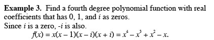
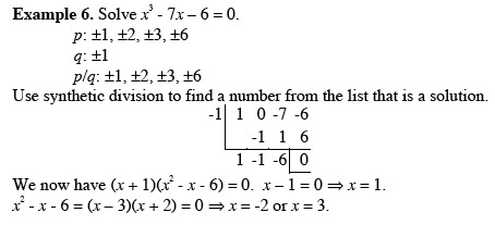
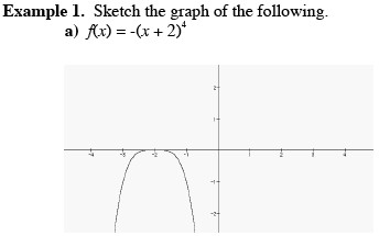
Example 3
Sketch the graph of the following on the same coordinate axis.
a) y = log₁₀x
Vertical asymptote x = 0
x-intercept (1, 0)
Additional point (10, 1)
b) y = log₁₀(x + 2)
Shift 2 units left from part a
Vertical asymptote x = -2
x-intercept (-1, 0)
Additional point (8, 1)
c) y = log₁₀(x + 2) - 1
Shift 2 units left and one unit down from part a
Vertical asymptote x = -2
Additional point (-1, -1)
x-intercept (8, 0)
Use graphing utility to verify results.

III. The Natural Logarithmic Function
The logarithmic function with base e [log_ex] is called the natural logarithmic function and is denoted by ƒ(x) = ln x.

Example 4: Evaluate
a) ln e⁵ = 5
b) e^{ln 3} = 3
c) ln (1 / e²) = ln e^-2 = -2

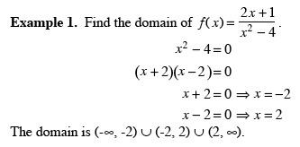
Example 5: find the domain of the following function.
ƒ(x) = ln (x + 3)
x + 3 > 0 => x > -3
The domain is (-3, ∞)

IV. Application

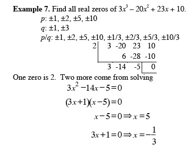
Example 7
The model
t = 12.5421 ln[x / (x - 1000)], x > 1000
approximates the length of a home mortgage of $150,000 at 8% in terms of the monthly payment. In the model, t is the length of the mortgage in years and x is the monthly payment in dollars. Find the length of the home mortgage of $150,000 at 8% if the monthly payment is $1300.
t = 12.4421 ln(1300 / 300) ≈ 18.4 years or 18 years and 5 months

This picture is from freeimages.co.uk.
It shows a typical American house. Many people use mortgages to purchase homes. The amount of time it takes to pay off a home can be calculated using a logarithmic function.

3.3 Properties of Logarithms
Objectives: Students will know how to rewrite logarithmic functions with a different base, use properties of logarithms to evaluate, rewrite, and expand expressions.
I. Change of Base
Our calculators have only two buttons for logarithmic functions, base 10 [log] and base e [ln]. To evaluate any other logarithmic functions using a calculator, we must rewrite it in one of these bases using the following formula.

Let a, b, and x be positive real numbers such that a ≠ 1 and b ≠ 1. Then
log_ax = log_bx / log_ba = log x / log a = ln x / ln a

Example 1: Evaluate the following
a) log₅18 = ln 18 / ln5 ≈ 1.7959
b) log₂42 = log 42/ log 2 ≈ 5.3923

II. Properties of Logartihms
Logarithms are exponents so the following properties are similar to exponent properties.

Let a be a positive real number such that a ≠ 1, let n be a real number, and let u and v be positive real numbers. Then
1. log_a(uv) = log_au + log_av
2. log_a(u/v) = log_au - log_av
3. log_auⁿ = n log_au

III. Rewriting Logarithmic Expressions

Example 2 Expand the logarithmic expression
a) log(2x³y⁴)
= log2 + logx³ + logy⁴
= log2 + 3logx + 4logy
b) ln [√(x+5) / y²] = ln√(x+5) - ln y² = (1/2) ln(x+5) - 2 ln y

Homework
p.236 -237
# 3 - 45 x 3's, 47 - 52 all, 54 - 60 x 3's, 73

Algebra I: Lesson Plan * 10/23/2006

Quickstart
MA.B.2.4.1 Practice #3 - 7

Lesson
1-9: Graphing Data on the Coordinate Plane Objective: To graph points on the coordinate plane, to analyze data using scatter plots, to interpret graphs in real-world situations

Graphing Points on the Coordinate Plane p.59
New vocabulary: coordinate plane, x-axis, y-axis, origin, quadrants, ordered pair, coordinates, x-coordinate, y-coordinate


Example 1: Identifying Coordinates p.60
Example 2: Graphing Points p.60
Check Understanding #1, 2
In which quadrant would you find each point from Check Understanding #2?

Analyzing Data Using Scatter Plots
Example 4: Making a Scatter Plot p.61
What correlation does the data in Example 4 show, positive, negative or none?

Chapter 5: Graphs and Functions 5-1 Relating Graphs to Events Objective: To interpret, analyze, and sketch graphs from real-world situations.
Chris's Adventure: Sketching a graph to model a real life situation.
Chris got up from his seat, walked slowly to the pencil sharpener, stopped and sharpened his pencil, walked slowly to the trash can, stopped to look out the window, the walked quickly back to his seat when Ms. Lynch called his name.

Interpreting, Sketching, and Analyzing Graphs p.236 - 237
Example 1: Interpreting Graphs
Check Understanding #1
Example 2: Sketching a graph
Check Understanding #2

Assignment
Green Workbook Section 1-9
Green Workbook Section 5-1

PreCalculus: Lesson Plan * 10/23/2006

Chapter 3: Exponential and Logarithmic Functions
3.1 Exponential Functions and their Graphs Objective: Students will be able to recognize, evaluate, and graph exponential functions.

IV. Compound Interest
A. Formulas for Compound Interest [p.222]
B. Finding the Balance for Compound Interest [p.223]

V. Other Applications
A. Population Growth [p.224]

This map is from the US census bureau website
www.census.gov/population/estimates/state/
The census allows the federal government to create models to predict changes in population.

Homework p. 227 #73, 74, 75 (algebraically)

PreCalculus: Lesson Plan * 10/18/2006

*PSAT Testing*

Review independently for Mid-term exam

Complete missing assignments

Pre-Read Chapter 3: Exponential and Logarithmic Functions

PreCalculus: Chapter 3 Essential Question

Chapter 3: Exponential and Logarithmic Functions

How can we analyze the similarities and differences between exponential and logarithmic functions graphically?

Algebra I: Lesson Plan * 10/13/2006

Pep Rally!

Buck Pride

PreCalculus: Lesson Plan * 10/13/2006

Quickstart
Sketch the graph of the functions on the same coordinate system.
ƒ(x)=e^x and g(x) = 1 + e^x

Assignment
In small groups, complete one problem from p.204 #14 - 28 even.
Use the Guidelines for Graphing Rational Functions [p.199]
and Asymptotes of a Rational Function [p.191] to assist your group.

Algebra I: Lesson Plan * 10/11/2006

Quickstart
p.209 #56 - 59

Lesson
4-5 Applying to Ratios to Probability Objective: To analyze real-world data, to find theoretical probability, and to find experimental probability.

I. Investigation p.210
"Understanding Probability"

II. Theoretical Probability
P(event) = (number of favorable outcomes) / (number of possible outcomes)

III. The Complement of an event
The complement of an event consists of all the outcomes not in the event.
The sum of the probabilities of an event and its complement is 1.
P(event) + P(not event) = 1
P(not event) = 1 - P(event)


IV. Experimental Probability
Probability based on data collected from repeated trials is experimental probability.
Experimental probability = (number of times an event occurs) / (number of times the experiment is done)

3 Example: Ryan flipped a quarter 6 times. The outcomes were 4 tails and 2 heads. So the experimental probability of getting heads is 2/6 or 1/3.

4-6 Probability of Compound Events
Independent events are events that do no influence one another.
If A and B are independent events,
P (A and B) = P(A) • P(B)


Homework
p.214 - 215 #3 - 45 x 3's

PreCalculus: Lesson Plan * 10/11/2006

Quickstart
1. Perform the indicated operation and write the result in standard notation.
( 4 - √-9)( 2 + √-9)
2. Write (3 + i)/i in standard form
3. Plot 6 - 5i and -3 + 2i in the complex plane.

Assignment
2.5 Group Quiz
In groups of 3 or 4, complete one problem from the following set p.187: 26, 28, 34, 36, 38

Lesson
2.6 Rational Functions and Asymptotes Objective: Students will know how to determine the domain and find asymptotes of rational functions

I Introduction to Rational Functions
a rational function is a function of the form ƒ(x) = N(x)/D(x), where N and D are both polynomials. The domain of ƒ is all x such that D(x) ≠ 0.


II. Horizontal and Vertical Asymptotes
A. Definition of asymptotes
1. The line x = a is a vertical asymptote of the graph of ƒ
if ƒ(x) approaches ±∞ as x approaches a, either from the right or left.
2.The line y = b is a horizontal asymptote of the graph of ƒ
if ƒ(x) approaches b as x approaches ±∞.
B. Asymptotes of Rational Functions Rules
Let ƒ be a rational function given by
ƒ(x) = N(x)/D(x)
= [a_nxⁿ + a_n-1x^n-1 + … + a₁x + a₀]/[b_mx^m + b_m-1x^m-1 + …+ b₁x + b₀].
1. The graph of ƒ has a vertical asymptote at x = a, if D(a) = 0 and N(a) ≠ 0.
2. The graph of ƒ has one horizontal asymptote or no horizontal asymptote, depending on the degree of N and D.
a. If n < m, y = 0
b. If n = m, y = a_n / b_m is the horizontal asymptote of the graph of ƒ.
c. n > m, then there is no horizontal asymptote of the graph of ƒ.


III Applications


2.7 Graphs of Rational Functions
Objective: Students will know how to sketch the graph of a rational function.

Guidelines for Graphing of Rational Functions [p. 199]
Let ƒ(x) = N(x)/D(x), where N(x) and D(x) are polynomials with no common factors.
1. Find and plot the y-intercept (if any) by evaluating ƒ(0).
2. Set the numerator equal to zero and solve the equation N(x) = 0. The real solutions represent the x-intercepts of the graph. Plot these intercepts.
3. Set the denominator equal to zero and solve the equation D(x) = 0. The real solutions represent the vertical asymptotes. Sketch these asymptotes using dashed vertical lines.
4. Find and sketch the horizontal asymptote of the graph using a dashed horizontal line.
5. Plot at least one point between and one point beyond each x-intercept and vertical asymptote.
6. Use smooth curves to complete the graph between and beyond the vertical asymptotes.

Homework
p.195 # 1 - 18 ALL
1 - 6, parts b and c only
7 - 12 are matching
13 - 18, parts a and b only

PreCalculus: Lesson Plan * 10/10/2006

Quickstart
Exploration p.169

Assignment
Writing about Math
p.176

Lesson
2.4 Complex Numbers (continued)
IV Plotting Complex Numbers
See Example 5 on p.178 in textbook

2.5 The Fundamental Theorem of Algebra Objective: Students will know how to find zeros of a polynomial function
I. The Fundamental Theorem of Algebra
A. The Fundamental Theorem of Algebra
If ƒ(x) is a polynomial of degree n, where n>0, then ƒ has at least one zero in the complex number system.
B. The Linear Factorization Theorem
If ƒ(x) is a polynomial function of degree n, where n>o, then ƒ has precisely n linear factors.


II. Conjugate Pairs
If ƒ is a polynomial function with real coefficients, then whenever a + bi is a zero of ƒ, a - bi is also a zero of ƒ.


III. Factoring a Polynomial
Every polynomial of degree n > 0 with real coefficients can be written as the product of linear and quadratic factors with real coefficients, where the quadratic factors have no real zeros.

ch2sec5c.jpg

Homework
p.185 - 187 # 5 - 50 x 5's

PreCalculus: Lesson Plan * 10/9/2006

Quickstart
1. Use synthetic division to determine if (x + #) is a factor of
f(x) = 3x³ + 4x² -18x - 3.
2. Divide using long division
(4x⁵ - x³ + 2x² - x) / ( 2x + 1 )
3. Use the Remainder Theorem to evaluate f(-3) for f(x) = 2x³ - 4x² + 1.

Lesson
2.3 Real Zeros of Polynomial Functions [continued]
Objective: Determine upper and lower bounds for zeros of polynomial functions.

V. Upper and Lower Bound Test
A way of dealing with a very large list generated by the Rational Zero Test is the Upper and Lower Bound Rule.
A real number b is an upper bound for the real zeros of f if there no zeros of f greater than b.
A real number b is a lower bound for the real zeros of f if there no zeros of f less than b.

Upper and Lower Bound Rule
Let f be a polynomial function with real coefficients and a positive leading coefficient. Suppose f(x) is divided by x – c using synthetic division.
1. If c > 0 and each number in the last row is either positive or zero,
then c is an upper bound for the real zeros of f.
2. If c < style="font-style: italic;">


2.4 Complex Numbers
Objective: Students will know how to perform operations with complex numbers and plot complex numbers in the complex plane.

I. Imaginary unit i
A. Definition
We need more numbers because simple equations such as x² + 1 = 0 do not have a real solution. We need a number whose square is –1.
i² = -1. i is called the imaginary unit.
By adding real numbers to multiples of the imaginary unit we get the set of complex numbers, defined as {a + bi | a is real, b is real and i² = -1}.
a + bi is the standard form for a complex number.
a is called the real part and bi is the imaginary part.
B. Two complex numbers a + bi and c + di are equal to each other if and only if a = c and b = d.

II. Operations with Complex Numbers
A. To add two complex numbers, we add the two real parts then add the two
imaginary parts. That is,
(a + bi) + (c + di) = (a + c) + (b + d )i


III. Complex Conjugates and Division
Two complex numbers in the form a + bi and a - bi are called complex conjugates.
(a + bi)(a - bi) = a² - (bi)² = a² + b².
We can use this fact to divide complex numbers.


Homework
p. 180 - 181 # 10 - 60 x 5's

Algebra I: Lesson Plan * 10/06/2006

Chapter 3 Test
Solving Inequalities

Practice Assignment
p.185 - 187 #5 - 60 x 5's
Finish for homework

Lesson
4-2 Proportions and Similar Figures
Objective: To find missing measures of similar figures and to use similar figures to measure indirectly
MA.B.1.4.3, MA.B.2.4.1

PreCalculus: Lesson Plan * 10/06/2006

Quickstart
1. Find all the zeros of f(x) = 6x⁴ - 33x³ - 18x².
2. Determine the right-hand and left-hand behavior of f(x) = 6x⁴ - 33x³ - 18x².
3. Find a polynomial function of degree 3 that has zeros of 0, 2, and -1/3

Lesson
(2.3) Real Zeros of Polynomial Functions
Objective: Students will know how to use long division and synthetic division to divide polynomials by other polynomials, determine the number of zeros of a polynomial, and find real zeros of polynomial function.

I. Long Division

The Division Algorithm



II. Synthetic Division


III. Remainder and Factor Theorems

Remainder Theorem



Factor Theorem



IV. The Rational Zero Test

PreCalculus: Lesson Plan * 10/05/2006

Quickstart
Exploration p.148

Lesson
(2.2) Polynomial Functions of Higher Degree
Objective: Students will know how to sketch and analyze graphs of polynomial functions.

I Graphs of Polynomial Functions
A. Characteristics
1. Polynomial functions are continuous. What this means to us is that the graphs of
polynomial functions have no breaks, holes, or gaps.
2. The graphs of polynomial functions have only nice smooth turns and bends. There are
no sharp turns as in the graph of y = |x|.
B.



C. Polynomial Functions are transformed in the same way as we discussed for cosine and sine functions. See example 1 in the textbook. (p.148)

The basic function is x^4. Because a = -1 it is reflected across the x-axis. Because -2 is subtracted inside the function, the graph is translated to the left 2 units.

II Leading Coefficient Test


III Zeros of Polynomial Functions
The following are equivalent statements, where f is a polynomial function and a is a real number. (p.151)
1. x = a is a zero of f.
2. x = a is a solution of the equation f(x) = 0.
3. (x – a) is a factor of f(x).
4. (a, 0) is an x-intercept of the graph of f.

Complete the Exploration on p.150
Part (a) has 3 zeros and 2 extrema, (b) 4 zeros and 3 extrema, (c) 3 zeros and 2 extrema.

It can be shown that for a polynomial function f of degree n, the following statements are true.
1. The graph of f has at most n real zeros.
2. The function f has at most n - 1 relative extrema (relative minimums or maximums).


Note that in the above example, 1 is a repeated zero. In general, a factor (x – a)k, k > 1, yields a repeated zero x = a of multiplicity k. If k is odd, the graph crosses the x-axis at x = a. If k is even, the graph only touches the x-axis at x = a.



IV. Intermediate Value Theorem

Let a and b be real numbers such that a < style="font-style: italic;">different signs.



Homework
Writing about Math
p. 155