Algebra I: Lesson Plan * 10/13/2006

Pep Rally!

Buck Pride

PreCalculus: Lesson Plan * 10/13/2006

Quickstart
Sketch the graph of the functions on the same coordinate system.
ƒ(x)=e^x and g(x) = 1 + e^x

Assignment
In small groups, complete one problem from p.204 #14 - 28 even.
Use the Guidelines for Graphing Rational Functions [p.199]
and Asymptotes of a Rational Function [p.191] to assist your group.

Algebra I: Lesson Plan * 10/11/2006

Quickstart
p.209 #56 - 59

Lesson
4-5 Applying to Ratios to Probability Objective: To analyze real-world data, to find theoretical probability, and to find experimental probability.

I. Investigation p.210
"Understanding Probability"

II. Theoretical Probability
P(event) = (number of favorable outcomes) / (number of possible outcomes)

III. The Complement of an event
The complement of an event consists of all the outcomes not in the event.
The sum of the probabilities of an event and its complement is 1.
P(event) + P(not event) = 1
P(not event) = 1 - P(event)


IV. Experimental Probability
Probability based on data collected from repeated trials is experimental probability.
Experimental probability = (number of times an event occurs) / (number of times the experiment is done)

3 Example: Ryan flipped a quarter 6 times. The outcomes were 4 tails and 2 heads. So the experimental probability of getting heads is 2/6 or 1/3.

4-6 Probability of Compound Events
Independent events are events that do no influence one another.
If A and B are independent events,
P (A and B) = P(A) • P(B)


Homework
p.214 - 215 #3 - 45 x 3's

PreCalculus: Lesson Plan * 10/11/2006

Quickstart
1. Perform the indicated operation and write the result in standard notation.
( 4 - √-9)( 2 + √-9)
2. Write (3 + i)/i in standard form
3. Plot 6 - 5i and -3 + 2i in the complex plane.

Assignment
2.5 Group Quiz
In groups of 3 or 4, complete one problem from the following set p.187: 26, 28, 34, 36, 38

Lesson
2.6 Rational Functions and Asymptotes Objective: Students will know how to determine the domain and find asymptotes of rational functions

I Introduction to Rational Functions
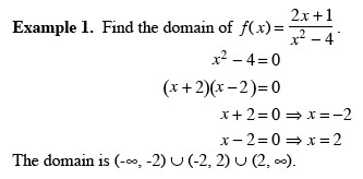
a rational function is a function of the form ƒ(x) = N(x)/D(x), where N and D are both polynomials. The domain of ƒ is all x such that D(x) ≠ 0.


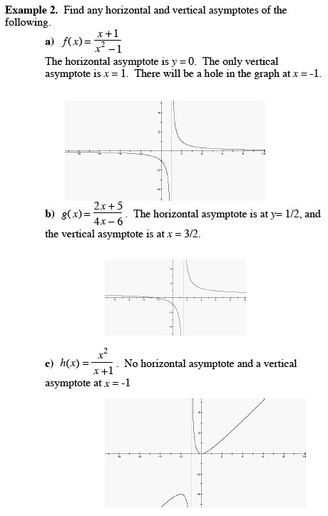
II. Horizontal and Vertical Asymptotes
A. Definition of asymptotes
1. The line x = a is a vertical asymptote of the graph of ƒ
if ƒ(x) approaches ±∞ as x approaches a, either from the right or left.
2.The line y = b is a horizontal asymptote of the graph of ƒ
if ƒ(x) approaches b as x approaches ±∞.
B. Asymptotes of Rational Functions Rules
Let ƒ be a rational function given by
ƒ(x) = N(x)/D(x)
= [a_nxⁿ + a_n-1x^n-1 + … + a₁x + a₀]/[b_mx^m + b_m-1x^m-1 + …+ b₁x + b₀].
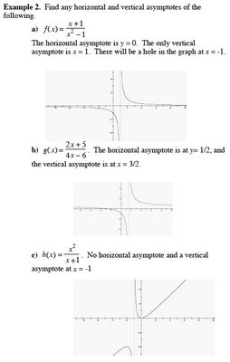
1. The graph of ƒ has a vertical asymptote at x = a, if D(a) = 0 and N(a) ≠ 0.
2. The graph of ƒ has one horizontal asymptote or no horizontal asymptote, depending on the degree of N and D.
a. If n < m, y = 0
b. If n = m, y = a_n / b_m is the horizontal asymptote of the graph of ƒ.
c. n > m, then there is no horizontal asymptote of the graph of ƒ.


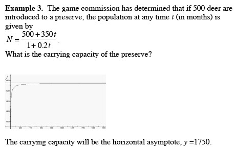
III Applications


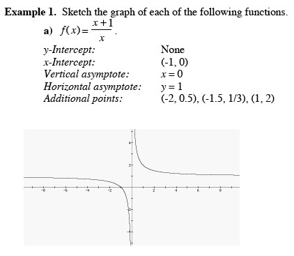
2.7 Graphs of Rational Functions
Objective: Students will know how to sketch the graph of a rational function.

Guidelines for Graphing of Rational Functions [p. 199]
Let ƒ(x) = N(x)/D(x), where N(x) and D(x) are polynomials with no common factors.
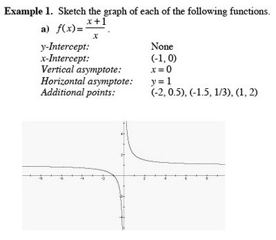
1. Find and plot the y-intercept (if any) by evaluating ƒ(0).
2. Set the numerator equal to zero and solve the equation N(x) = 0. The real solutions represent the x-intercepts of the graph. Plot these intercepts.
3. Set the denominator equal to zero and solve the equation D(x) = 0. The real solutions represent the vertical asymptotes. Sketch these asymptotes using dashed vertical lines.
4. Find and sketch the horizontal asymptote of the graph using a dashed horizontal line.
5. Plot at least one point between and one point beyond each x-intercept and vertical asymptote.
6. Use smooth curves to complete the graph between and beyond the vertical asymptotes.

Homework
p.195 # 1 - 18 ALL
1 - 6, parts b and c only
7 - 12 are matching
13 - 18, parts a and b only

PreCalculus: Lesson Plan * 10/10/2006

Quickstart
Exploration p.169

Assignment
Writing about Math
p.176

Lesson
2.4 Complex Numbers (continued)
IV Plotting Complex Numbers
See Example 5 on p.178 in textbook

2.5 The Fundamental Theorem of Algebra Objective: Students will know how to find zeros of a polynomial function
I. The Fundamental Theorem of Algebra
A. The Fundamental Theorem of Algebra
If ƒ(x) is a polynomial of degree n, where n>0, then ƒ has at least one zero in the complex number system.
B. The Linear Factorization Theorem
If ƒ(x) is a polynomial function of degree n, where n>o, then ƒ has precisely n linear factors.


II. Conjugate Pairs
If ƒ is a polynomial function with real coefficients, then whenever a + bi is a zero of ƒ, a - bi is also a zero of ƒ.


III. Factoring a Polynomial
Every polynomial of degree n > 0 with real coefficients can be written as the product of linear and quadratic factors with real coefficients, where the quadratic factors have no real zeros.

ch2sec5c.jpg

Homework
p.185 - 187 # 5 - 50 x 5's

PreCalculus: Lesson Plan * 10/9/2006

Quickstart
1. Use synthetic division to determine if (x + #) is a factor of
f(x) = 3x³ + 4x² -18x - 3.
2. Divide using long division
(4x⁵ - x³ + 2x² - x) / ( 2x + 1 )
3. Use the Remainder Theorem to evaluate f(-3) for f(x) = 2x³ - 4x² + 1.

Lesson
2.3 Real Zeros of Polynomial Functions [continued]
Objective: Determine upper and lower bounds for zeros of polynomial functions.

V. Upper and Lower Bound Test
A way of dealing with a very large list generated by the Rational Zero Test is the Upper and Lower Bound Rule.
A real number b is an upper bound for the real zeros of f if there no zeros of f greater than b.
A real number b is a lower bound for the real zeros of f if there no zeros of f less than b.

Upper and Lower Bound Rule
Let f be a polynomial function with real coefficients and a positive leading coefficient. Suppose f(x) is divided by x – c using synthetic division.
1. If c > 0 and each number in the last row is either positive or zero,
then c is an upper bound for the real zeros of f.
2. If c < style="font-style: italic;">


2.4 Complex Numbers
Objective: Students will know how to perform operations with complex numbers and plot complex numbers in the complex plane.

I. Imaginary unit i
A. Definition
We need more numbers because simple equations such as x² + 1 = 0 do not have a real solution. We need a number whose square is –1.
i² = -1. i is called the imaginary unit.
By adding real numbers to multiples of the imaginary unit we get the set of complex numbers, defined as {a + bi | a is real, b is real and i² = -1}.
a + bi is the standard form for a complex number.
a is called the real part and bi is the imaginary part.
B. Two complex numbers a + bi and c + di are equal to each other if and only if a = c and b = d.

II. Operations with Complex Numbers
A. To add two complex numbers, we add the two real parts then add the two
imaginary parts. That is,
(a + bi) + (c + di) = (a + c) + (b + d )i


III. Complex Conjugates and Division
Two complex numbers in the form a + bi and a - bi are called complex conjugates.
(a + bi)(a - bi) = a² - (bi)² = a² + b².
We can use this fact to divide complex numbers.


Homework
p. 180 - 181 # 10 - 60 x 5's

Algebra I: Lesson Plan * 10/06/2006

Chapter 3 Test
Solving Inequalities

Practice Assignment
p.185 - 187 #5 - 60 x 5's
Finish for homework

Lesson
4-2 Proportions and Similar Figures
Objective: To find missing measures of similar figures and to use similar figures to measure indirectly
MA.B.1.4.3, MA.B.2.4.1